Ad:
THREE RESERVOIRS PROBLEM AND PIPE NETWORK
Branched pipes: Three Reservoirs Problem
 |
| Fig: Branched pipes: three inter connected Reservoir |
In water supply system, Often a number of reservoirs are required to be interconnected by means Of a pipe system consisting of a number of pipes namely main and branches which meet at a junction. Figure shows three reservoirs 'B' and 'C' are interconnected by pipes 'a', 'b' and 'c' which meet at a junction 'D'.
In the problem Of this type lengths, diameters and friction factors Of the different pipes are supposed to be known. Further it is assumed that the flow is steady, minor losses are small and hence neglected and the reservoirs are large enough so that their water surface levels are constant (i.e. velocity at reservoir surface levels are constant).
Three basic equations namely, Continuity equation,
Bernoulli's equation and Darcy — Weisbach equation are used in order to solve
the problem. According to the continuity equation at any junction we observe that amount of liquid flowing into the junction is equal to the amount of liquid flowing out.
Let 'Da', 'Db' and 'Dc' be the diameters; 'La', 'Lb' and 'Lc' be the lengths; 'Qa', and 'QC' be the discharges; 'Va', 'Vb,' and 'Vc' be the velocities of flow in the pipes 'a', 'b' and 'c' respectively. Now, if 'Pd/γ' be the pressure head at the junction (D); 'Z', and 'C ' are respectively the heights of the water surfaces in the reservoirs 'A', 'B' and 'C'; 'Z/ is the height of junction 'D' above the assumed datum and 'hfa', 'hfb' and 'hfc' be the head losses due to friction in the pipes 'a', 'b' and 'c' respectively. Assume, 'Z' =
![]()
(i) CASE - 1: [Zj> Zb; Water will flow from 'A' to 'D' and 'D' to both 'B' & 'C'

Qlnflow to Junction(D)= QOutflow from Junction (D)

Now, Applying Continuity equation, We get
Types of problems in three reservoirs system and their solution

Step 3: Find 'Qb' from equation (XIV) with the known values of 'Zj', 'Zb', and 'rb'
Step 4: Find 'Qc' form equation (XVI) with the known values of 'Qa' and 'Qb'
Step 5: Find 'Zc' form equation (XV) with the known values of 'Zj' 'rc', and 'Qc'.
Step 6: If the values of 'Qb' & 'Qc' seem to be negative then it is conformed that the assumed flow direction in Step 1 is altered having the same magnitude of 'Qb' & 'QC'

Step 3: Find 'Qa' & 'QC' after solving the equations (XX) and (XXI) with the known values of 'Qb', 'Za', 'ra', 'Zc' and 'rc'.
Step 4: Find 'Zj' form equation (XXI) with the
known values of 'Za' 'ra and 'Qa' ('Zc' or 'rc' and 'Qc').
Step 5: Find Zb form equation (XVIII) with the known values of 'Zj' 'rb' and 'Qb' .
Step 6: If the values of 'Qa' & 'Qc' seem to be
negative then it is conformed that the assumed flow direction in Step I is
altered having the same magnitude of 'Qa' & 'Qc'.

Solution:
(A) Analytical method:
Step 1: Let us assume CASE - I: [Zj>Zb; Water will flow
from 'A' to 'D' and 'D' to both 'B' & 'C']
Step 2: Write the Energy and Continuity equations.

Step 3: Find 'Qa' from equation (XXII) with the known values
of 'Zj', 'Za' & 'ra'.
Step 4: Find 'Qc' from equation (XXIV) with the known values
of 'Zj', 'Zc' & 'rc'.
Step 5: Find 'hfa' & 'hfc' with the known values of 'ra',
'rc', 'Qa' & 'QC'. Now, if 'hfa' & 'hfc' are positive then it is
conformed that the assumed flow direction in Step 1 is correct but if they are
negative then the assumed flow direction in Step 1 is not correct; so the flow
direction should be changed.
Step 6: Choose the actual flow direction in pipes 'a', 'b'
and 'c' from the following chart,

Step 7: Suppose the flow direction in pipes 'a', 'b' and 'c'
is as Case (P). So, write the Energy and Continuity equations corresponding to
Case (P).

Step 8: Suppose, Qc=mQb. Now, from equation (XXIX), Qa=(1+m)Qb
Step 9: Equating equations (XXVI) and (XXVII) Za-raQa2 = Zb+ rbQb2

Now, find the value of 'm' from the equation (XXXII) with the
known values of 'ra' 'rb', 'rc', 'Za', 'Zb' and 'Zc'
Step 11: Find 'Q,' from equation (XXX); and finally 'Qa'
& 'QC' from Step 8.
Ad:
https://happyshirtsnp.com/
(B) Trial
and Error method:
Step 1: Same procedure is carried out from Step 1 to Step 7 of Analytical method.
Step 2: Assume, 741 = (Za + Zc)/2 and find the required value of 'Qa', 'Q/ & 'QC' from the following table by judging the value of 'Z' side by side as in the figure below.
|
z |
hfa |
hfb |
hfc |
|
|
|
∑Qj= Qa -(Qb +Qc) |
|
zjl |
hfal |
hfb1 |
hfc1 |
Qa1 |
|
Qc1 |
x |
|
zj2 |
hfa2 |
hfb2 |
hfc2 |
Qa2 |
Qb2 |
Qc2 |
|
|
zj3 |
hfa3 |
hfb3 |
hfc3 |
Qa3 |
Qb3 |
Qc3 |
z |
|
|
|
|
|
|
|
|
|
|
jn |
hfan |
hJbn |
hfcn |
Qan |
Qbn |
Qcn |
|

Now, repeat the procedure until '∑Qj = (Qa —(Qb +Qc)) = 0' and get the final value of discharges in pipe 'a', 'b' & 'c' as ' Qan', ' & ' Qcn .
Regarding the choosing the value of 'Z', takes in increasing order if initially '∑Qj = (Qa -(Qb +Qc))' is positive and takes in decreasing order if initially '∑Qj =(Qa-(Qb +Qc))' is negative.
Introduction to Pipe Networks Problem
 |
| Fig: Pipe network |
A group of interconnected pipes forming several loops (or
circuits) is called a pipe networks. Such networks of pipes can be seen common in municipal water distribution system in cities.
Main problem in a pipe network is to determine the
distribution of flow through the various pipes of the network such that all the
conditions of flow are satisfied and all the loops (or circuits) are then
balanced.
The conditions to be satisfied in any network of pipes are
as follows;
i) Principle of continuity:
The flow into each junction must be equal to the flow out of
the junction. For example;
At
junction 'H': QCH + QGH = QHD + QHE + QHF
At junction 'A': QI = QAG + QAB
(ii) Principle of energy:
In each loop (or circuit), the loss of head due to flow in
Clockwise (C/W) direction must be equal to the loss of head due to flow in
Anticlockwise (AC/W) direction. For example;
In loop 'ABCHGA': hfAB + hfBC + hfCH
= hfHG + hfGA
In loop 'CDHC': hfCD = hfDH
+ hfHC
(iii) Darcy - Weisbach equation:
This equation must be satisfied for flow in each pipe. Minor
losses are neglected if the pipe lengths are large enough. However, if the
minor losses are large, they may be taken into account by considering them in
terms of the head loss due to friction in equivalent pipe length.
We know, Darcy-Weisbach equation,

Where, 'n' is an exponent having a numerical value ranging
from 1.72 to 2.0.
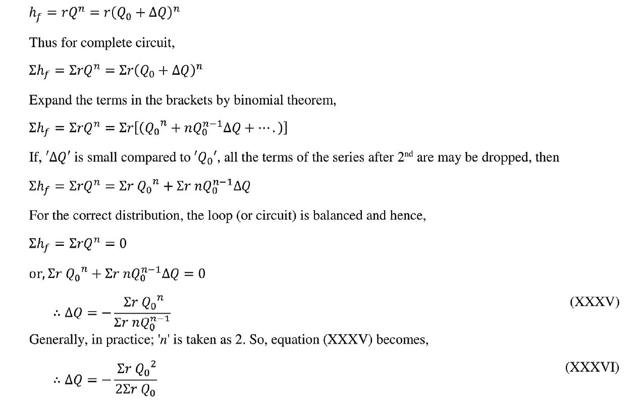
Derivation for correction (∆Q):
For any pipe, if 'Q0' is the assumed discharge then correct discharge is
Q=Q0+∆Q
Now, from the above equations we get;
Hardy Cross method of solving of pipe network problems
The pipe network problems are in general complicated and
can't be solved analytically. As such method of successive approximation are
utilized. "Hardy cross" method is commonly used to solve such problems. It can solve complex pipe
network forming a loop (or circuit) and the approach is head balance approach.
Procedure for the solution of network problem:
(i)
Assume, suitable rate of flow (i.e. Q0) and its
direction of flow in each pipe in such a way that continuity equation at each
junction should be satisfied.
(ii)
Compute head losses (hf) = 'rQ0 2 '
and 'rQ0' for each pipe with the help of 'Qo'.
(iii) For each loop, determine the algebraic sum of head losses as ∑hf = ∑rQ0 2 . Consider head losses from C/W flow as +ve and from AC/W flow as -ve.
(iv) For each loop (or circuit), determine; ∑rQo. But, here; sum is calculated without considering the sign (i.e. take absolute value).
(v) For each loop (or circuit), determine; '∆Q' as, ∆Q = -∑r Qo 2 /2∑r Qo.
vi) For each pipe, determine; (Q) as, Q = Q + ∆Q. If '∆Q' = +ve, then add it to the flow in C/W direction and subtract it from the flow in AC/W direction. If '∆Q' = -ve, then add it to the flow in AC/W direction and subtract it from the flow in C/W direction.
(vii) For the pipes common to two loop (or circuit), a correction is applied from the both loops.
(viii) Use the corrected flow for the next trial.
(ix) Repeat the steps from (i) to (Viii) until the correction (∆Q) becomes negligible.
Comments
Post a Comment