
Reynold's Experiment | Laminar flow's in circular pipe | Shear stress distribution

  Reynold's Experiment

• Osborne Reynolds (Mathematician & Physicist, UK)

• In 1883, he developed a laboratory set up in which he injected Dye (i.e. a fine, threadlike stream of colored liquid having the same density as water) at the entrance to a large glass tube through which water was flowing from a tank.


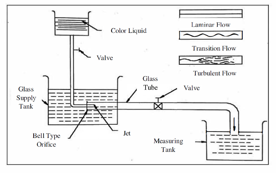
Fig: Reynold's experiment


Ad:


• Procedure:

✓ The water from the tank was allowed to flow through glass tube into atmosphere.

✓ The velocity of flow was varied by the valve.

✓ Dye was injected into the flow through a small tube.

• Observation:

✓ At the initial stage of flow, dye filament in the glass tube was in the form of straight line. This was a laminar flow.

✓ When increasing the velocity of flow, the dye filament was no longer a straight line. The dye filament starts to become wavy. This was a transitional flow.

✓ While further increase in velocity of flow, the wavy dye filament broke up and finally diffused in water. This was a turbulent flow.

✓ The occurrence of a laminar and turbulent flow was governed by the relative magnitude of inertia and viscous force. For low velocities, viscous force is predominant whereas for higher velocities, inertia force is predominant.
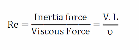


Where,

V= Mean velocity, u= Coefficient of Kinematics viscosity = μ/p,

μ= Coefficient of Dynamic viscosity = up, p= Density of fluid,

L = Characteristics length, L= Diameter of Pipe (D), in pipe flow


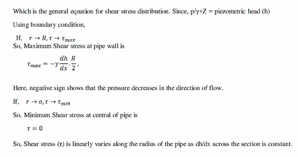
Laminar Flow in Circular Pipe

Assumptions: incompressible, steady, developed laminar flow in a circular pipe.

A horizontal pipe of radius 'R' through which a fluid of density 'p' flows.

Let us consider, a fluid element with having radius 'r' of length 'dx' in the direction of flow.

Here,

p = Pressure intensity

't= Shear stress on the periphery of the cylinder acting in opposite direction of flow.

Forces acting on the fluid element: Pressure force, Shear force and Component of weight.

Fig: Forces acting on a fluid element


Ad:


Ad:


Comments

Popular posts from this blog

Use of double mass curve analysis | Test for the consistency of records (Double mass curve)

Use of double mass curve analysis The double mass curve is used to check the consistency of many kinds of hydrological data by comparing data for a single station with that of pattern composed of the data from the several other station in the area. The double mass curve can be used to adjust inconsistent precipitation data. The theory of double mass curve is based upon the fact that a plot of the two cumulative quantities during the same period exhibit a straight line so long as the proportionality between the two remains unchanged and the slope of the line represent the proportionality. This method can be smooth at a time series and suppress random elements in the series. In recent 30 yrs, Chinese scholars analyzed the effects of soil and water conservation measures and land use/cover changes on runoff and sediments using double mass curve method and have achieved the good results. In this study, double-mass curves of precipitation vs sediments are plotted for the two contrastive peri...

Nikuradse experiment | variation of frictional factor (f) for laminar and turbulent flow

  Nikuradse', a German Engineer, He by gluing uniform sand grains on the inner side of the pipe wall to artifically roughened the pipe conducted a series of well- planned experiments on pipes. Here we choose the pipe of different diameter (D) and by changing the size of sand grain which gives (Roughness height= k), We can observe from his experiment that value of (k/D) varies from about "1/1014 to 1/30"  Since from dimensional analysis 'f is the function of Reynold's no VD/ ν  and ratio of 'k/D' Where, k =Average roughness height of pipe wall, D= Diameter of pipe,   ν = Kinematic viscosity of flowing fluid, Re =VD/ ν  = Reynold's no, k/D = Relative roughness.  Sometimes, "k/D" is also replaced by "R/k" Where, R= Radius of pipe and (R/k)= Relative smoothness whose value varies from "15 to 507''. Ad: Change(Variation) of friction factor for laminar flow (Re<2000) Head loss in laminar flow (i.e. Hagen-Poisseullie equati...

Hydrodynamically smooth and rough boundaries | Velocity distribution for turbulent flow

 Hydrodynamically smooth and rough boundaries Fig: Definition of smooth and rough boundaries In general, a boundary with irregularities of large average height 'K' on its surface is considered to  be a rough boundary and one with smaller 'K' value is considered as a smooth boundary. ✓ However, for a proper classification of smooth and rough boundaries, the flow and fluid characteristics are required to be considered in addition to the boundary characteristics. ✓ As the flow outside the laminar sub-layer is turbulent, eddies of various sizes are present which try  to penetrate through the laminar sublayer. But, due to greater thickness of laminar sub-layer ,   eddies can't reach the surface irregularities and thus the boundary acts as a smooth boundary. Such  a boundary is termed as " Hydro-dynamically Smooth Boundary" ✓ With the increase in Reynold's no (Re), the thickness of the laminar sub-layer  decreases and it's  can even become much smaller ...