Velocity distribution in smooth pipes
In the vicinity of a smooth boundary there exists a laminar sublayer. The flow in the laminar sublayer being laminar has a parabolic velocity distribution. Since the thickness of laminar sublayer (δ') is generally very small, the parabolic velocity distribution in the region may be approximated by a straight line without appreciable error.
So, in the zone of laminar sublayer, since the flow is laminar, the viscous stress predominates and the turbulent stresses tend to become zero. Therefore, in the laminar sublayer, the shear is

For linear velocity distribution within the laminar sublayer, 'du/dy' becomes 'u/y'.
Ad:
 |
| Fig: Velocity distribution for turbulent flow near a smooth boundary |
Furthermore, if it is assumed that in the laminar sublayer, i.e. up to y=δ', 'τ' remains constant and equal to 'τo'. The shear stress at the pipe boundary is

Which is the velocity distribution laminar number sublayer, i.e. form y=0 to y=δ'. Here, term (u* y/u) is dimensionally to a form of Reynold's number
Form Nikuradse's experiment of turbulent flow in smooth pipe,


Which represents the velocity distribution in the region of turbulent flow near hydrodynamically smooth boundaries and it is applicable for regions outside the laminar sublayer i.e. y≥δ'.
Velocity distribution in rough pipes
The flow condition near hydrodynamically rough boundaries are different from that of hydrodynamically smooth boundaries. This is so because in the case of rough boundaries the surface irregularities protrude well behind the laminar sub layer, which is therefore is completely destroyed as shown in fig. As such velocity distribution in turbulent flows near hydrodynamically rough boundaries is considerably affected by the surface protrusions eqn applies equally to the turbulent flow in hydrodynamically rough pipes.
In order to obtain the equation which would represent the velocity distribution for turbulent flow near hydrodyamically rough boundaries is considerably affected by surface protrusions(k), y' must be evaluated in terms of the average height of the surface
protrusions (k).
So, from Nikuradse's experiment for rough boundary, y' α k, :. y' = k/30
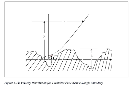 |
| Fig: Velocity distribution for turbulent flow near rough boundary |

Which represent the velocity distribution for the turbulent flow near hydrodynamically rough boundary.
Ad:

- Pipe flows and open channel flows in Hydraulics
Reynold's Experiment | Laminar flow's in circular pipe | Shear stress distribution
Interception and Interception losses
Turbulent Flow | Velocity and shear stress in turbulent flow
Reynold's Theory | Prandtl mixing length Theory
Hydrodynamically smooth and rough boundaries | Velocity distribution for turbulent flow
Nikuradse experiment | variation of frictional factor (f) for laminar and turbulent flow
- Determination of Value of 'f' from Moody's Chart
Minor head losses in pipes | Equivalent length of pipe representing minor head losses
Comments
Post a Comment