
Determination of Value of 'f' from Moody's Chart | Hydraulics

 Moody's Diagram (or Moody's Chart)


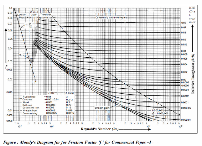
Fig: Moody's diagram for the friction factor 'f' for commercial pipes-I


L.F. Moody has plotted the equation as shown in above figures, commonly known as 'Moody Diagram' which is essentially the same as thet of Nikuradse's plot except for the transition regions. So, 'Moody chart' is the chart of friction factor 'f' versus 'Re' curves for various values of 'R/k'.
For any turbulent pipe flow problem the value of friction factor (f) can therefore be determined from
Moody's Diagram  if the numerical values of 'R/k' for the pipe and 'Re' of flow are known. The values of 'k' which may be adopted for the pipes of some of the common materials are given below


Ad:

Fig: Moody's diagram for friction factor 'f' for commercial pipes-II


The value of Equivalent sand grain roughness (k)' given in Table 1-2 correspond to material in new and clean condition. As the pipe become older, the roughness increases may increase with time in accordance with following expression


Where, k= Equivalent sand grain roughness at any time 't', Equivalent sand grain roughness of new pipe material and a = Time rate of increase of roughness.

Salient features of Moody's Diagram

a) Laminar flow (Re<2000)

Friction factor (f) is a function of 'Re' only


b)                Critical zone (2000<Re<4000)

Flow in this zone is either laminar or turbulent (i.e. oscillatory flow that alternately exists between laminar and turbulent flow). There is no any specific relationship between 'f 'and 'Re' in this zone.


c)                Transition zone (Re>4000)

For 'k/D < 0.001 ' and certain ranges of 'Re' in this zone, the roughness elements are submerged in the viscous sub-layer, and the flow can be considered to be smooth pipe flow. In this zone, T is a function of both 'Re' and 'k/D'.


d)                Complete turbulent zone (Re>4000)


In this zone, average roughness height is substantially greater than the viscous wall layer thickness. As 'Re' is high, the head loss is also higher due to the extra turbulence caused by projections. The friction factor (f) is a function of 'k/D' only and is independent of 'Re'. The horizontal lines indicate that friction factor (D does not change with 'Re', that means viscosity does not affect the head loss in this zone.


Determination of Value of 'f' from Moody Chart:


(i)               Mark the value of 'Re' =VD/v on the abscissa (i.e. Re - axis)

(ii)             For the given value of 'k/D', mark the point of intersection of 'Re' with 'k/D'. To find the intersection point, draw vertical line from 'Re' and follow curve path from 'k/D'. If 'k/D' curve is not available for given value of 'k/D', draw a curve by following the trend of nearby curve.

iii) Draw a horizontal line from the point of intersection of 'Re' and 'k/D' to ordinate (i.e. f- axis) 

(iv)               Finally, read the value of friction factor (D from the chart.


                                                 Flow chart of Friction factor (f)

Flow chart for friction factor 'f'


Friction factor (f) can be calculated either from Resistance Equations or by using Moody Chart as in Figure. When Moody Chart is not given then use the Resistance Equations to calculate the friction factor (f).


Ad:


Read more:


Comments

Popular posts from this blog

Use of double mass curve analysis | Test for the consistency of records (Double mass curve)

Use of double mass curve analysis The double mass curve is used to check the consistency of many kinds of hydrological data by comparing data for a single station with that of pattern composed of the data from the several other station in the area. The double mass curve can be used to adjust inconsistent precipitation data. The theory of double mass curve is based upon the fact that a plot of the two cumulative quantities during the same period exhibit a straight line so long as the proportionality between the two remains unchanged and the slope of the line represent the proportionality. This method can be smooth at a time series and suppress random elements in the series. In recent 30 yrs, Chinese scholars analyzed the effects of soil and water conservation measures and land use/cover changes on runoff and sediments using double mass curve method and have achieved the good results. In this study, double-mass curves of precipitation vs sediments are plotted for the two contrastive peri...

Nikuradse experiment | variation of frictional factor (f) for laminar and turbulent flow

  Nikuradse', a German Engineer, He by gluing uniform sand grains on the inner side of the pipe wall to artifically roughened the pipe conducted a series of well- planned experiments on pipes. Here we choose the pipe of different diameter (D) and by changing the size of sand grain which gives (Roughness height= k), We can observe from his experiment that value of (k/D) varies from about "1/1014 to 1/30"  Since from dimensional analysis 'f is the function of Reynold's no VD/ ν  and ratio of 'k/D' Where, k =Average roughness height of pipe wall, D= Diameter of pipe,   ν = Kinematic viscosity of flowing fluid, Re =VD/ ν  = Reynold's no, k/D = Relative roughness.  Sometimes, "k/D" is also replaced by "R/k" Where, R= Radius of pipe and (R/k)= Relative smoothness whose value varies from "15 to 507''. Ad: Change(Variation) of friction factor for laminar flow (Re<2000) Head loss in laminar flow (i.e. Hagen-Poisseullie equati...

Hydrodynamically smooth and rough boundaries | Velocity distribution for turbulent flow

 Hydrodynamically smooth and rough boundaries Fig: Definition of smooth and rough boundaries In general, a boundary with irregularities of large average height 'K' on its surface is considered to  be a rough boundary and one with smaller 'K' value is considered as a smooth boundary. ✓ However, for a proper classification of smooth and rough boundaries, the flow and fluid characteristics are required to be considered in addition to the boundary characteristics. ✓ As the flow outside the laminar sub-layer is turbulent, eddies of various sizes are present which try  to penetrate through the laminar sublayer. But, due to greater thickness of laminar sub-layer ,   eddies can't reach the surface irregularities and thus the boundary acts as a smooth boundary. Such  a boundary is termed as " Hydro-dynamically Smooth Boundary" ✓ With the increase in Reynold's no (Re), the thickness of the laminar sub-layer  decreases and it's  can even become much smaller ...